

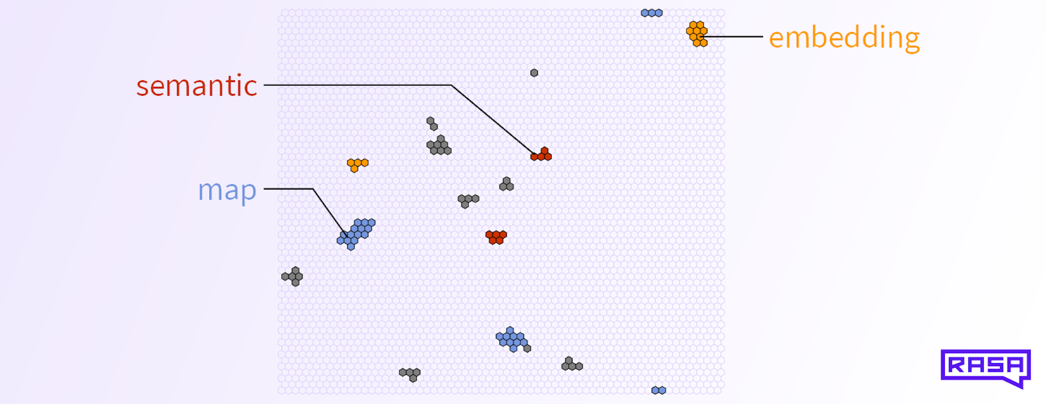


In Part I we introduced semantic map embeddings and their properties. Now it's time to see how we create those embeddings in an unsupervised way and how they might improve your NLU pipeline.
Training Semantic Maps
At the heart of our training procedure is a batch self-organizing map (BSOM) algorithm. The BSOM takes vectors as training inputs and essentially arranges them in a grid such that similar vectors end up close to each other.
Sorting Colors
To visualize the BSOM process better, let's forget about text and natural language processing for the moment, and pretend that we want to arrange colors in a two dimensional grid such that similar colors are neighbouring. Our input vectors are therefore three-dimensional RGB color vectors with entries between 0 and 1.

Let's say we want to arrange the 10 colors shown above into a 12 ⨉ 12 grid. The BSOM algorithm first creates a 12 ⨉ 12 matrix where the entries are random vectors of the size of the input, i.e. 3. The resulting (12, 12, 3) tensor is often called the "codebook". Since our inputs are RGB colors, this tensor is also a 12 ⨉ 12 pixel image, specifically, the image shown in the top left corner of the figure below.

The BSOM algorithm looks at each color in the training data and decides which unit in the codebook (the "pixels") has a color that is most similar to that input. Once it has identified all these best matching pixels, it goes through each of the 144 pixels in the codebook and assigns a weighted average of training colors to that pixel, where the weights depend on how far the best matching pixel of the input is from the current pixel. The closer the best matching pixel of an input is to the current pixel, the more weight is given to it.
This process is repeated many times, and each time the radius of influence decreases. You can see how the codebook changes in each step in the image above.
Since we had only 10 training colors and the map has 12 ⨉ 12 = 144 pixels, every input is nicely separated from every other input after training is complete. Note that every color in the training data appears in the final image, and it is close to similar colors (e.g. pink and purple are in the top right corner and the greens are in the lower left corner).
The shape of the resulting color clusters depends on how we define the distance between pixels, as this distance enters the weights of the weighted sum. (For illustration purposes we set pixels that are not influenced by any input to black, so the shapes are clearly visible. Normally, pixels would retain the color that was last assigned to them, and thus the colored clusters would be connected by interpolated colors.) In the instance above, we use the Chessboard distance, and as a result we see squares of colors in the final image. Alternatively we can use a hexagonal distance function that also wraps around at the edges (the left edge is connected to the right, and the top edge to the bottom):

This can help with convergence when inputs have more than three dimensions and leads to the hexagonal grid look that you saw throughout Part I of this post.
All of this also works when we have more inputs than pixels on the map.
So, a BSOM has only a few hyperparameters to tune: the map width and height, the number of training epochs, the choice of pixel-distance function, and perhaps some parameters that determine how quickly the radius of influence decreases in each epoch.
Adapting the BSOM to Text
To adapt the BSOM algorithm to natural language processing, we use high-dimensional binary vectors as inputs instead of RGB colors. Each input vector now represents one snippet of text from some text corpus, such as Wikipedia or this very blog post. Each binary entry in the vector is associated with one word in a fixed vocabulary, and it is 1 if the word appears in the snippet and otherwise 0. In essence, each input is now a binarized bag-of-words vector.
If we use a structured corpus such as this blog post as training data, we use paragraphs as snippets and also prepend all the respective title words to each snippet. So the previous paragraph becomes a vector where the entries for "To", "adapt", "the", "BSOM", ... are 1, but also "Adapting", "to", "Text" and "Training", "Semantic", "Maps", as well as "Exploring", "Map", "Embeddings" from the title of this blog post.
We then use the binary bag-of-words vectors of the snippets to train the BSOM algorithm. We have implemented a fast parallelized version that is specialized to binary input vectors, so we can train on all of Wikipedia in a day or two for a 128 ⨉ 128 map and 79649 words in the vocabulary.
Extracting the Embeddings from the Codebook
The BSOM algorithm results in a dense codebook tensor. We can think of it as a M ⨉ N matrix where each entry is a real vector whose size is the size Nvocab of the vocabulary. What do these vocabulary-sized vectors represent? At the end of the BSOM training, each component of these vectors is the weighted average of 1s and 0s of inputs that are associated with that pixel. In other words, the _k_th entry in each codebook vector represents the probability that the _k_th word in the vocabulary appears in the context that is represented by that codebook vector!
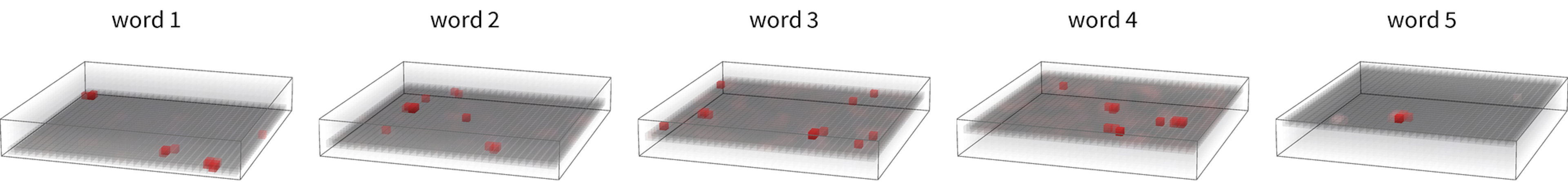
To create the semantic map embedding for the _k_th word, we consider the _k_th slice of our trained M ⨉ N ⨉ Nvocab codebook. This slice is a M ⨉ N matrix where each pixel in that matrix represents a context class, and the value of each pixel represents the probability that the _k_th word appears in that context class. We illustrate this matrix on the left side of the figure below. To create our sparse embedding we set the 98% of all pixels with the lowest values to zero, as shown in the center of the figure. The 98% value is arbitrary, but it should be close to 100%, as we wish to generate sparse matrices. Finally, we set all the remaining non-zero values to 1. The resulting sparse binary matrix is a simplified form of our semantic map embedding for the _k_th word.

All pixels that are 1 signify that this word appears particularly often in the context classes associated with those pixels. Alternatively, we can also normalize the codebook and divide the pixel values in the _k_th codebook slice by the probability of any word appearing in a context class. As a result, we get 1s for context classes where the word appears particularly often compared to other words. This, in fact, is our default.

We can repeat that process for each word in our vocabulary to generate embeddings for all words in the vocabulary.
Semantic Maps in the Rasa NLU Pipeline
Semantic map embeddings have some very interesting properties, as we've seen in Part I of this post. But do they help with NLU tasks such as intent or entity recognition? Our preliminary tests suggest that they can help with entity recognition, but often not with intent classification.
For our tests we feed our semantic map embedding features into our DIET classifier and run intent and entity classification experiments on the ATIS, Hermit (KFold-1), SNIPS, and Sara datasets. The figure below compares the weighted average F1 scores for both tasks on all four datasets and compares them with the scores reached using BERT or Count-Vectorizer features:

We observe that our Wikipedia-trained (size 128 ⨉ 128, no fine-tuning) semantic map embedding reaches entity F1 scores about half way between those of the Count-Vectorizer and BERT. On some datasets, the semantic map that is trained on the NLU dataset itself (no pre-training) can also give a performance boost. For intents, however, semantic map embeddings seem to confuse DIET and are outperformed even by the Count-Vectorizer, except on the Hermit dataset.
Having said this, when we feed the semantic map features into DIET, we do not make use of the fact that similar context classes are close to each other on the map and that might be the very key to make this embedding useful. We've got plenty of ideas of where to go from here, but we thought it is a good point to share what we're doing with this project. Here are some of the ideas:
- Instead of DIET, use an architecture that can make use of the semantic map embedding properties to do intent and entity classification. For example, a Hierarchical Temporal Memory (HTM) algorithm or the architectures explored here.
- When training on Rasa NLU examples, let the BSOM algorithm only train on prepended intent labels during the first epoch, and afterwards on the intent labels and the text.
- Use a max-pooling layer to reduce the representation's size.
- Explore text filtering / bulk-text-labelling based on the binary features.
- Create semantic maps for other languages.
If you are curious and want to try out the Semantic Map embedding for yourself, we've created a SemanticMapFeaturizer component for the Rasa Open Source 2.x! You can find the featurizer on the NLU examples repo. It can load any pre-trained map that you find here. Let us know how this works for you (e.g. you can post in the forum and tag @j.mosig)!